
Response to Risk in an Investment Simulation
You may have already played the investment simulation game on the front page of my website. If you haven’t, I highly encourage you to try it at least once before reading further! You’ll start with $1.00 and you will be able to enter your money in and out of the S&P 500 over a random 5-year period. At the end of the 5-year period you can compare your performance with the market (if you entered your money in the market at the start and never sold) and other visitors to my website. My advice: put your money in when you think the market will go up, and take it out when you think the market will go down.
Scroll down to read more when you’ve finished!

Ok! Welcome back! So a few confessions:
- Although it is technically random which 5-year period you experienced when you played the game, the set of possible 5-year periods you could have been assigned to contains only three such periods: 1986-1991, 1996-2001, and 2007-2012. While allowing for any set would certainly be possible, I wanted to allow visitors to directly compare their performance to the performance of others on an apples to apples basis (i.e., experiencing the exact same 5-year period)… and I don’t expect to get enough site visitors to provide adequete sample sizes for every such combination.
- My advice, that you should put your money in when you think the market will go up, and take it out when you think the market will go down, I wholeheartedly stand by. However, it may be a bit misleading. On expectation, without literally knowing what will happen next, the market is always more likely to go up than go down. Therefore, another way to interpret my advice is that you should put your money in the market and never take it out. This doesn’t outperform the market (it literally is the market) and it won’t outperform every other visitor to the site (as some will get lucky with a more active strategy), but its probably the optimal strategy for maximizing earnings. But I can’t blame you for not being super motivated to maximize a fake dollar by doing nothing…
If you’d like to learn more about how I created this game using d3.js, check out the github repository.
How did people do?
As of May 1st 2018, there had been 783 completed simulations of the S&P 500 by visitors to the site (“players”). Since a player could have completed the same 5-year period multiple times, I restricted the data to only the first time each period was played by a given player (i.e., a player may have up to three completed simulations in the data - one for each period). This resulted in 647 total completed simulations, with approximately 215 simulations per period. The simulation moves in 1 week intervals for a total of 260 intervals per period.
| Period | Count |
|---|---|
| April 11, 1986 - March 28, 1991 | 214 |
| December 13, 1996 - November 30, 2001 | 215 |
| September 7, 2007 - August 24, 2012 | 218 |
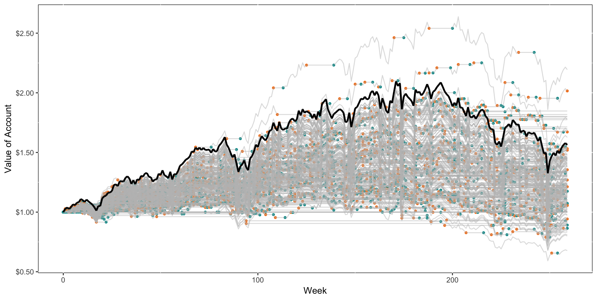
On each of the following charts, the black line indicates the actual performance of the market, and the grey lines indicates the performance of each individual player. Aqua dots indicate buys and orange dots indicate sells.
April 11, 1986 - March 28, 1991

Summary of Performance
Over this period the market earned 59%, while players only earned an average of 34%.
82% of players performed worse than the market with the worst performer actually losing 15%!
16% of players performed better than the market with the best performer earning an astounding 108%! Congrats to that lucky anonymous player - you (may) know who you are!
Predictors of Success
I ran a simple linear regression to see how two attributes of a simulation predicted overall performance. First, I calculated the number of total trades for each player across the period (to measure how active the player was), and second, I calculated in which week the player first entered the market.
| Estimate | Std. Error | t value | Pr(>|t|) | |
|---|---|---|---|---|
| (Intercept) | 1.381 | 0.020 | 67.563 | 0.000 |
| totalTrades | -0.001 | 0.001 | -2.734 | 0.007 |
| firstTrade | -0.001 | 0.001 | -1.801 | 0.073 |
While both trading more frequently and waiting to enter the market made players worse off, the main culprit appears to be active trading.
December 13, 1996 - November 30, 2001
Summary of Performance
Over this period the market earned 56%, while players only earned an average of 24%.
92% of players performed worse than the market with the worst performer actually losing 32%!
7% of players performed better than the market with the best performer earning a ridiculous 119%! Also, congrats to that lucky anonymous player - who appears to be different than the player who crushed the prior period.
Predictors of Success
I ran a simple linear regression to see how two attributes of a simulation predicted overall performance. First, I calculated the number of total trades for each player across the period (to measure how active the player was), and second, I calculated in which week the player first entered the market.
| Estimate | Std. Error | t value | Pr(>|t|) | |
|---|---|---|---|---|
| (Intercept) | 1.296 | 0.021 | 61.016 | 0.000 |
| totalTrades | 0.000 | 0.001 | -0.815 | 0.416 |
| firstTrade | -0.003 | 0.000 | -5.088 | 0.000 |
Active trading didn’t seem to hurt performance here - but waiting too long to enter was extremely problematic. Given the early increase of the market and the late decline, this is not surprising.
September 7, 2007 - August 24, 2012
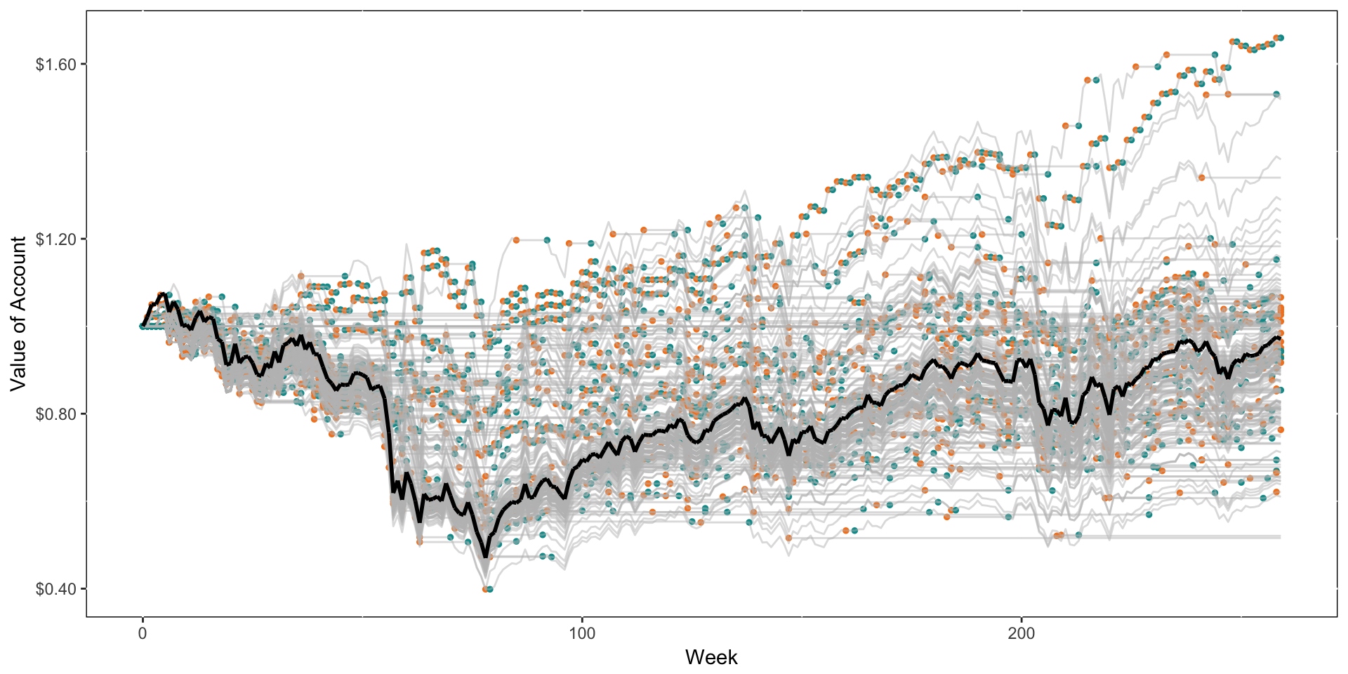
Summary of Performance
Over this period the market actually went down - it lost 3%, while players didn’t generally perform any better with an average loss of 7%.
68% of players performed worse than the market with the worst performer losing 48%.
28% of players performed better than the market with the best performer earning 66%! The best performing players stayed out of the market early and entered it to ride the inceasing wave late.
Predictors of Success
I ran a simple linear regression to see how two attributes of a simulation predicted overall performance. First, I calculated the number of total trades for each player across the period (to measure how active the player was), and second, I calculated in which week the player first entered the market.
| Estimate | Std. Error | t value | Pr(>|t|) | |
|---|---|---|---|---|
| (Intercept) | 0.905 | 0.013 | 72.152 | 0.000 |
| totalTrades | 0.001 | 0.000 | 4.211 | 0.000 |
| firstTrade | 0.001 | 0.001 | 1.752 | 0.081 |
Given that the market went down over this 5-year period (a rare occurence over the history of the S&P 500), active trading was actually a crucial component to performing well! Waiting to enter the market was also marginally predictive of performance - once again not too surprising given the early decline and late boom.
Conclusion
In general, players performed quite poorly relative to the market. This was even true when the market went down, and was especially true when the market went up. In general, its simply hard to predict what will happen next! This is consistent with data from the real world - that outperforming the market is difficult (and requires luck) while consistently outperforming the market is nearly impossible (Malkiel 1973). Reiterating my advice from the beginning, put your money in the market (ideally in a low cost index fund), and sit back and relax.

Predicting Trades
While the market is clearly hard to predict, is the trading behavior of players? In a given simulation, players experienced 260 weeks and for each of these 260 weeks they made 260 discrete choices. For each week that the player was already in the market, they chose between exiting the market and staying in it. For each week that the player was not in the market, they chose between entering the market and staying out of it. Can each choice be predicted by their past choices and market movements?
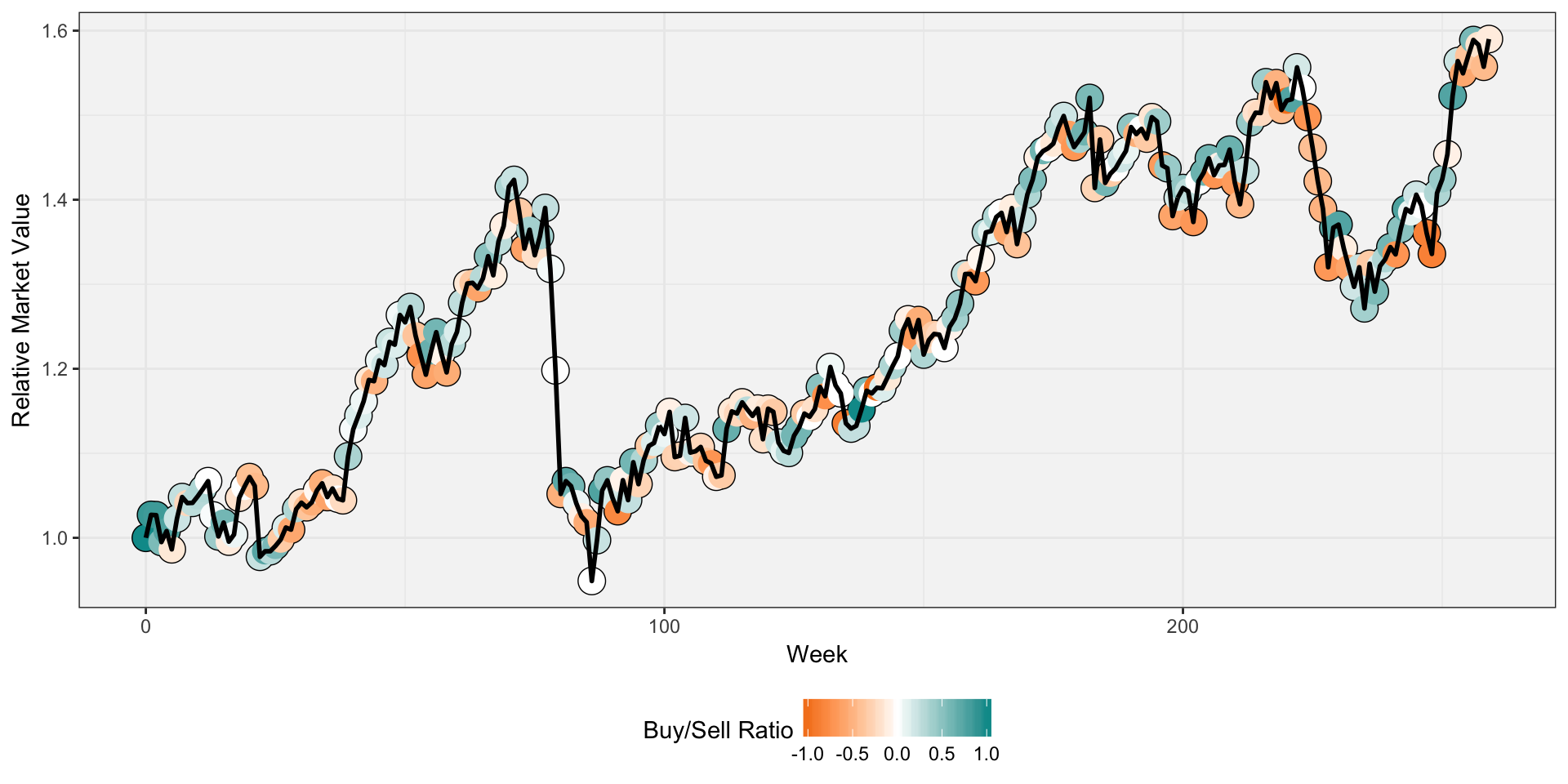
Below are graphs for each period showing whether a given week was relatively more of a buying week or a selling week. For each week, the percent of trades that were a buy (instead of a sell) were calculated and normalized so a score of 1 refers to 100% buys, a score of -1 refers to 100% sells, and a score of 0 refers to 50% buys and 50% sells. This score was encoded to a color spectrum from aqua to orange, where darker aqua points are more heavily buying weeks and darker orange points are more heavily selling weeks. Lighter versions of either color express a more balanced week, with pure white representing 50/50.
April 11, 1986 - March 28, 1991
December 13, 1996 - November 30, 2001

September 7, 2007 - August 24, 2012
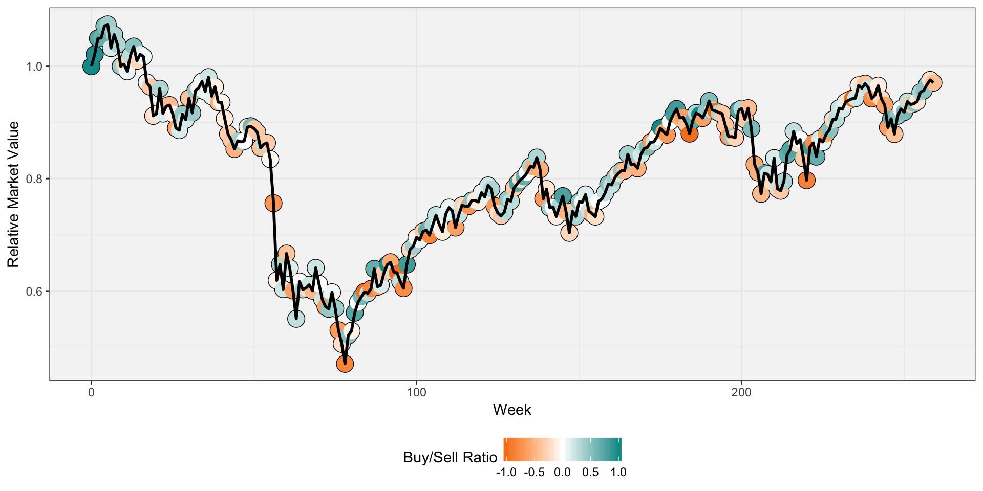
The graphs look pretty noisy, but a clear pattern seems to emerge. At local minimums on the graph, players tend to sell more, and at local maximums on the graph, players tend to buy more. This is of course precisely what a player would not want to do! From a predictive standpoint, this suggests that perhaps players are responding to the recent past performance of the market - getting out when it just took a downturn and getting in when it just started to go up.
To statistically analyze this, I used individual level data where the unit of observation is a given week for a given simulation/player. With 647 simulations and 260 weeks per simulation, this led to an overall dataset of 168,220 observations. I further divided the data into two groups: weeks where players entered the week in the market (predicting sells) and weeks where players entered the week out of the market (prediciting buys).
In general, players tended to be in the market - there were 100,932 weeks (60.2%) where players were in the market and chose between selling and staying in, and 67,288 weeks (39.8%) where players were not in the market and chose between buying and staying out.
I created a number of new features to include in a predictive model:
period: Which simulation the player was in.week: The week number of the simulation (from 1 to 260).Lag_1: The percent increase or decrease in the market since the previous week.Lag_2: The percent increase or decrease in the market since two weeks prior.Lag_5: The percent increase or decrease in the market since five weeks prior.Lag_10: The percent increase or decrease in the market since ten weeks prior.totalTrades: The total number of trades the player had made up to that point.weeksSinceTrade: The total number of weeks since the player had last traded.perfSinceTrade: The percent increase or decrease in the market since the player last traded.valueRelI: The percent increase or decrease since the start of the simulation.valueRelM: The percent increase or decrease relative to the market (i.e., had the player bought in week 1 and held).
Predicting Sells
Among players in the market, I ran a logistic regression predicting whether a player chose to sell (= 1) or not sell (= 0). In addition to including all the above features as fixed effects, I also included a random effect for each player, to control for individual differences.
| Estimate | Std. Error | z value | Pr(>|z|) | |
|---|---|---|---|---|
| (Intercept) | -2.372 | 0.118 | -20.115 | 0.000 |
| period1996-12-13 | 0.003 | 0.044 | 0.071 | 0.943 |
| period2007-09-07 | -0.325 | 0.056 | -5.789 | 0.000 |
| week | -0.004 | 0.000 | -13.719 | 0.000 |
| Lag_1 | -4.711 | 0.793 | -5.938 | 0.000 |
| Lag_2 | -7.717 | 0.682 | -11.310 | 0.000 |
| Lag_5 | 0.961 | 0.428 | 2.244 | 0.025 |
| Lag_10 | 1.483 | 0.271 | 5.467 | 0.000 |
| totalTrades | 0.034 | 0.001 | 51.575 | 0.000 |
| weeksSinceTrade | -0.026 | 0.001 | -29.425 | 0.000 |
| perfSinceTrade | 1.180 | 0.168 | 7.029 | 0.000 |
| valueRelI | -0.180 | 0.108 | -1.662 | 0.096 |
| valueRelM | 0.368 | 0.132 | 2.795 | 0.005 |
The significant negative coefficients of Lag_1 and Lag_2 suggest that players in the market are more likely to sell if the market has just gone down in the short-term, but the significant positive coefficient of Lag_10 suggests that they are more likely to sell if the market has gone up in the mid-term. It seems that the immeadiate response to a dip in the market is to sell, but a solid trend of upward movement means its times to lock in the gains.
Similarly, the significant positive coefficient of perfSinceTrade also shows evidence of a disposition effect. Players who have seen the market rise since they entered the market want to lock in their gain and chalk it up as a net positive - poentially without considering the positive benefits of remaining in the market.
Predicting Buys
Among players not in the market, I ran a logistic regression predicting whether a player chose to buy (= 1) or not buy (= 0). In addition to including all the above features as fixed effects, I also included a random effect for each player, to control for individual differences.
| Estimate | Std. Error | z value | Pr(>|z|) | |
|---|---|---|---|---|
| (Intercept) | -1.559 | 0.122 | -12.770 | 0.000 |
| period1996-12-13 | -0.327 | 0.046 | -7.034 | 0.000 |
| period2007-09-07 | 0.137 | 0.066 | 2.082 | 0.037 |
| week | -0.008 | 0.000 | -23.918 | 0.000 |
| Lag_1 | 6.864 | 0.736 | 9.322 | 0.000 |
| Lag_2 | 4.140 | 0.640 | 6.473 | 0.000 |
| Lag_5 | -0.565 | 0.433 | -1.305 | 0.192 |
| Lag_10 | -0.798 | 0.283 | -2.818 | 0.005 |
| totalTrades | 0.033 | 0.001 | 49.873 | 0.000 |
| weeksSinceTrade | -0.030 | 0.001 | -22.744 | 0.000 |
| perfSinceTrade | 1.270 | 0.229 | 5.553 | 0.000 |
| valueRelI | 0.190 | 0.121 | 1.569 | 0.117 |
| valueRelM | -0.142 | 0.145 | -0.982 | 0.326 |
The significant positive coefficients of Lag_1 and Lag_2 suggest that players out of the market are more likely to sell if the market has just gone up in the short-term, but the significant negative coefficient of Lag_10 suggests that they are more likely to sell if the market has gone down in the mid-term. Mirroring that of sells, it seems that the immeadiate response to a rise in the market is to buy and not miss out, but a solid trend of downward movement means its times to jump in and hope for a turnaround (or perhaps because entering the market seems like a good deal).
Interestingly, similar to sells, there is a significant positive coefficient of perfSinceTrade. This suggests that buyers are more likely to enter the market if it has gone up since they last sold. Instead of being stubborn and letting the inertia of a bad decision kick in, players seem to be taking action on their regret and jumping back in the market even if they missed out on some solid gains. This is of course counteracted by a significant negative coefficient of weeksSinceTrade as players becomes increasingly less likely to re-enter the market the longer they have gone since selling. The high correlation between these two variables makes it tricky to disentangle them and form any clear inferential conclusions.